Introduction

Statement: All the datasets on the server are computed by a standard pipeline and are compatible with each other. Use the Google Chrome browser for best visualization quality.

GEPIA is a web server for analyzing the RNA sequencing expression data of 9,736 tumors and 8,587 normal samples from the TCGA and the GTEx projects, using a standard processing pipeline.

Quick start

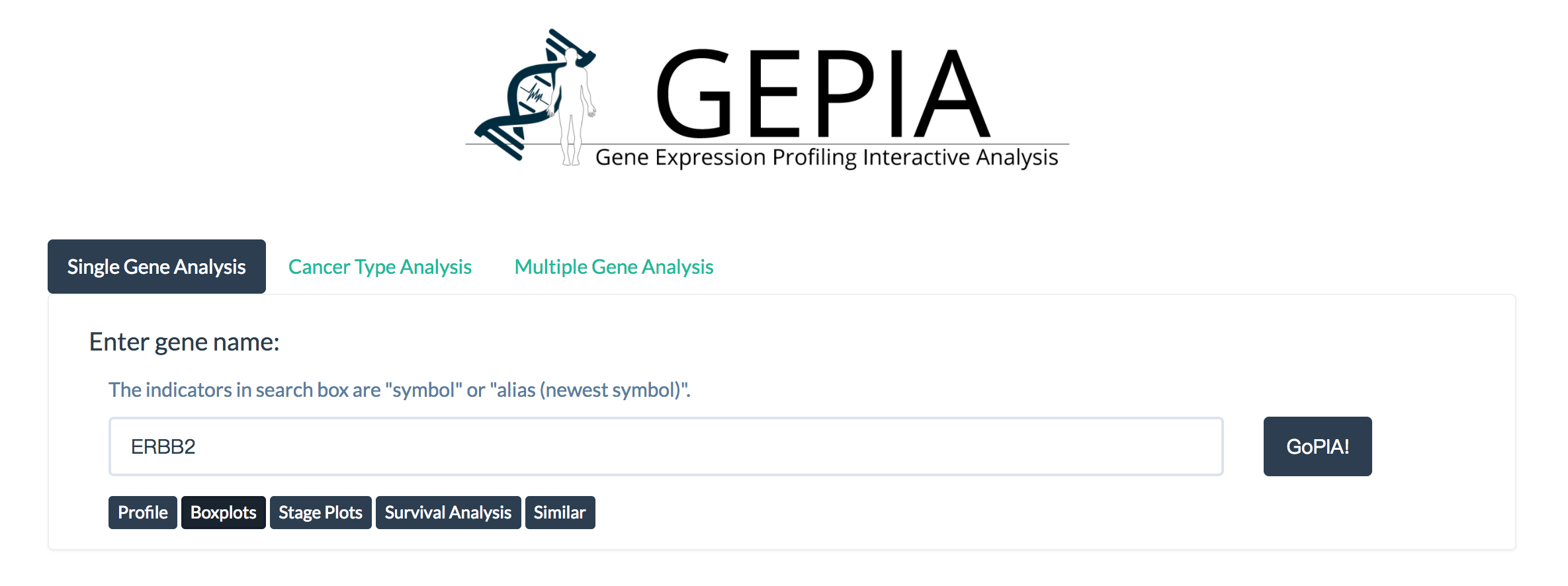
Enter a gene symbol or gene ID (Ensembl ID) in the “Enter gene name" field, and click the “GoPIA!" button to search for the gene of interest.

Features

Differential Expression Analysis

This feature allows users to apply custom statistical methods and thresholds on a given dataset to dynamically obtain differentially expressed genes and their chromosomal distribution.

Parameters

Dataset: Select a cancer type of interest.
Chromosome Distribution: Select “Over-expressed”, “Under-expressed” or “Both” for chromosomal distribution plots.

Differential thresholds: [See detail of differential analysis methods here]

Differential Methods: Select a method for differential analysis.
|log₂FC| Cutoff: Set custom fold-change threshold.
q-value Cutoff: Set custom q-value threshold.
Percentage Cutoff: Set custom percentage threshold.

For the ANOVA and LIMMA options, genes with higher |log₂FC| values and lower q values than pre-set thresholds are considered differentially expressed genes.

For the Top 10 option, genes with higher log₂FC values and higher percentage value than the thresholds are considered over-expressed genes; thus, only over-expressed genes will be presented in the list and the chromosomal plot.

Results

Differential genes

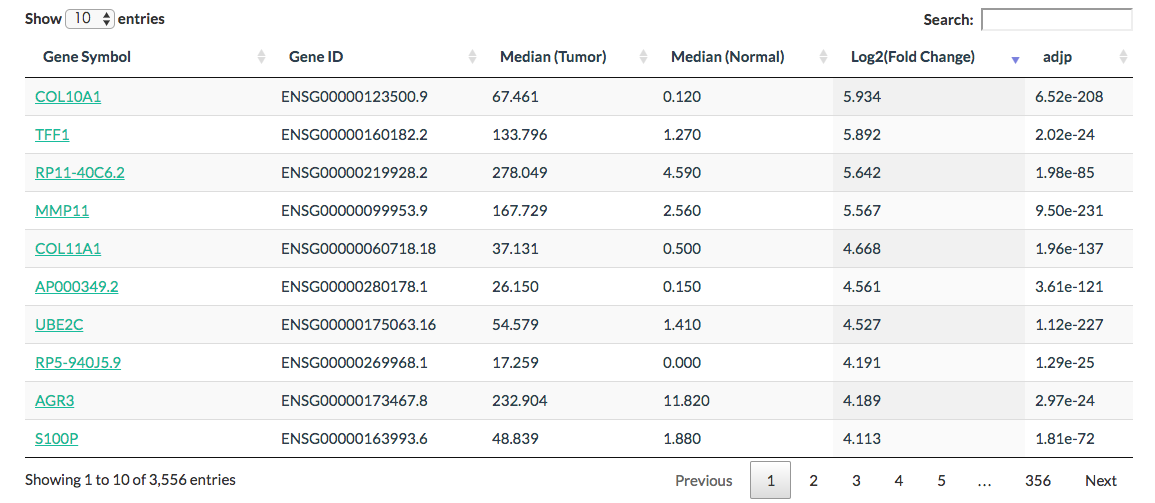
Click the “List” button: GEPIA will generate a list of differentially expressed genes [by default, the list sorted in descending order of log₂FC] based on input parameters.

Chromosomal distribution plots

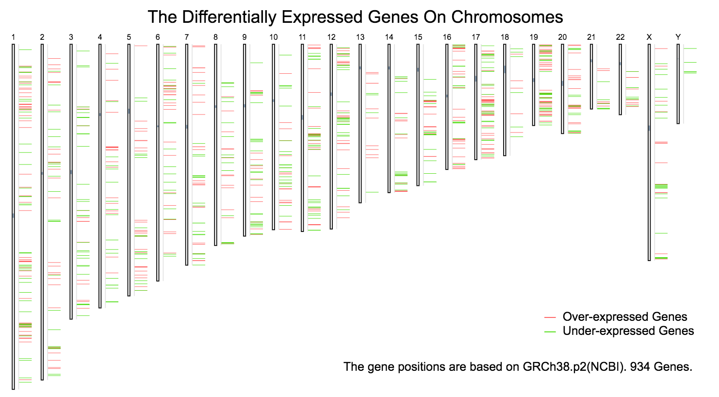
Click the “Plot” button: GEPIA will generate a chromosomal distribution plot. The over-expressed genes in chromosome are marked by red lines, while under-expressed genes are marked green.

DIY Expression

GEPIA plots expression profiles of a given gene according to selected datasets and statistical methods by cancer types or pathological stages. The details are shown below:

Gene Expression Profile

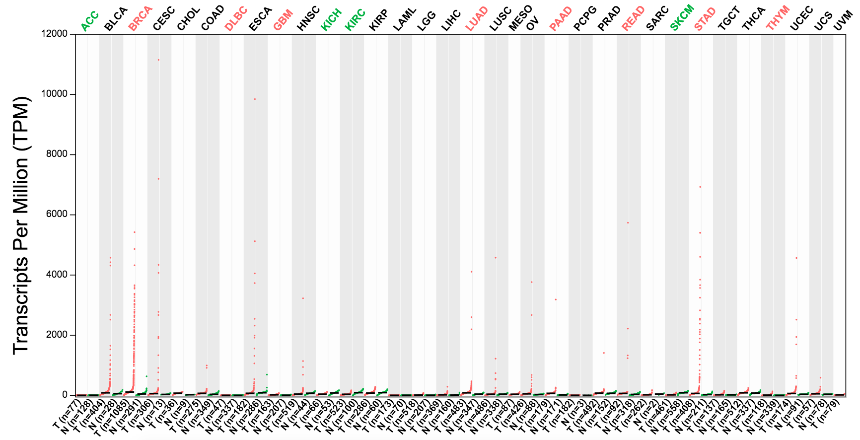
GEPIA generates dot plots profiling gene expression across multiple cancer types and paired normal samples, with each dot representing a distinct tumor or normal sample.

Parameters

Gene: Input a gene of interest.
Dataset/Tissue Order: Select cancer types of interest in the “Dataset” field and click “add” or “all” to build a dataset list in the “Tissue Order” field. Manual input of cancer types split by comma (e.g. ACC,BRCA,BLCA) is also acceptable. The x-axis of the plot will follow the order of datasets.
Log Scale: Choose whether to use linear or log₂(TPM + 1) transformed expression data for plotting.
Matched Normal data: Select “TCGA normal + GTEx normal”, “Only TCGA normal” or “None” for matched normal data in plotting. [The matched normal samples for differential analysis are “TCGA normal + GTEx normal”]
Plot Width: Set custom plot width.

Differential thresholds: [See detail of differential analysis methods here]

Differential Methods: Statistical methods used for differential gene expression analysis.
|log₂FC| Cutoff: Set custom fold-change threshold.
q-value Cutoff: Set custom q-value threshold.
Percentage Cutoff: Set custom percentage threshold.

For the ANOVA and LIMMA options, genes with higher |log₂FC| values and lower q values than pre-set thresholds are considered differentially expressed genes.

For the Top 10 option, genes with higher log₂FC values and higher percentage value than the thresholds are considered over-expressed genes.

Results

Click the “Plot” button: GEPIA will generate a gene expression profile based on users’ custom input parameters.

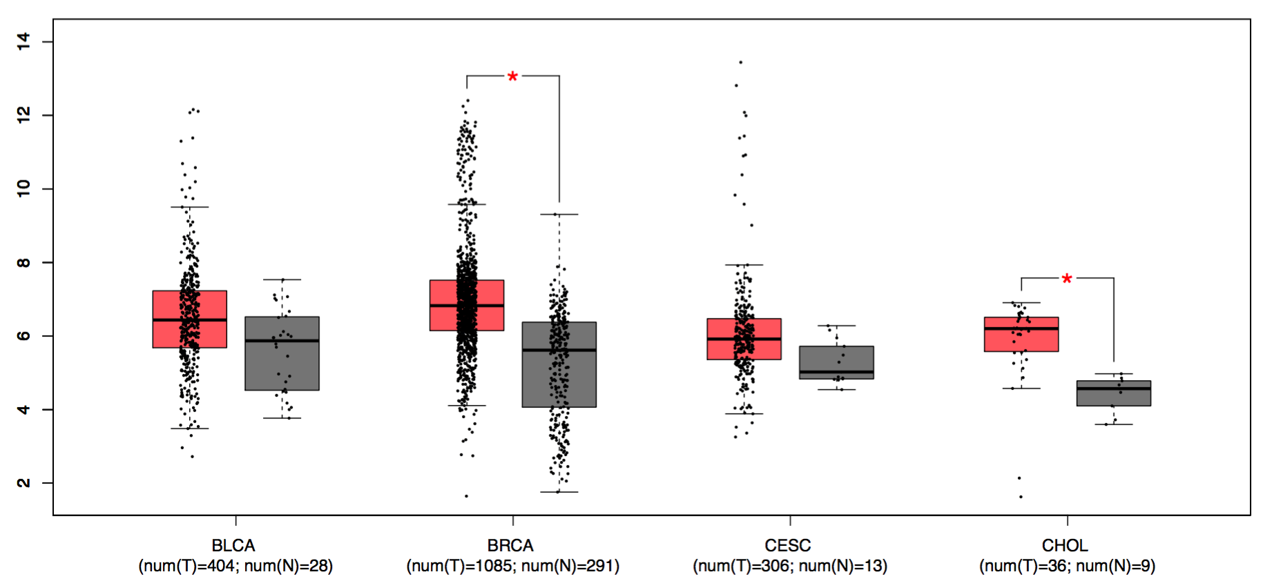
Box Plots

GEPIA generates box plots with jitter for comparing expression in several cancer types (For best visual quality, we recommend 1-4 cancer types).

Parameters

Gene: Input a gene of interest.
Datasets Selection/Dataset: Select cancer types of interest in the “Dataset Selection” field and click “add” to build a dataset list in the “Dataset” field. Manual input of cancer types split by comma (e.g. ACC,BRCA,BLCA) is also acceptable. The x-axis of the plot will follow the order of datasets.
Tumor Color: Set the box color of tumor dataset.
Normal Color: Set the box color of normal dataset.
Log Scale: Choose whether to use linear or log₂(TPM + 1) transformed expression data for plotting.
Jitter Size: Set the size of jitter across the box.

Differential thresholds:

|log₂FC| Cutoff: Set custom fold-change threshold.
p-value Cutoff: Set custom p-value threshold.
Matched Normal data: Select “TCGA normal + GTEx normal”, “Only TCGA normal” for differential analysis and plotting.

The differential analysis here is based on the selected datasets (“TCGA tumors vs TCGA normal + GTEx normal” or “TCGA tumors vs TCGA normal”). The method for differential analysis is one-way ANOVA, using disease state (Tumor or Normal) as variable for calculating differential expression:

Gene expression ~ disease state

The expression data are first log₂(TPM+1) transformed for differential analysis and the log₂FC is defined as median(Tumor) - median(Normal).

Genes with higher |log₂FC| values and lower q values than pre-set thresholds are considered differentially expressed genes.

Results

Click the “Plot” button: GEPIA will present a gene expression box plot based on users’ custom input parameters.

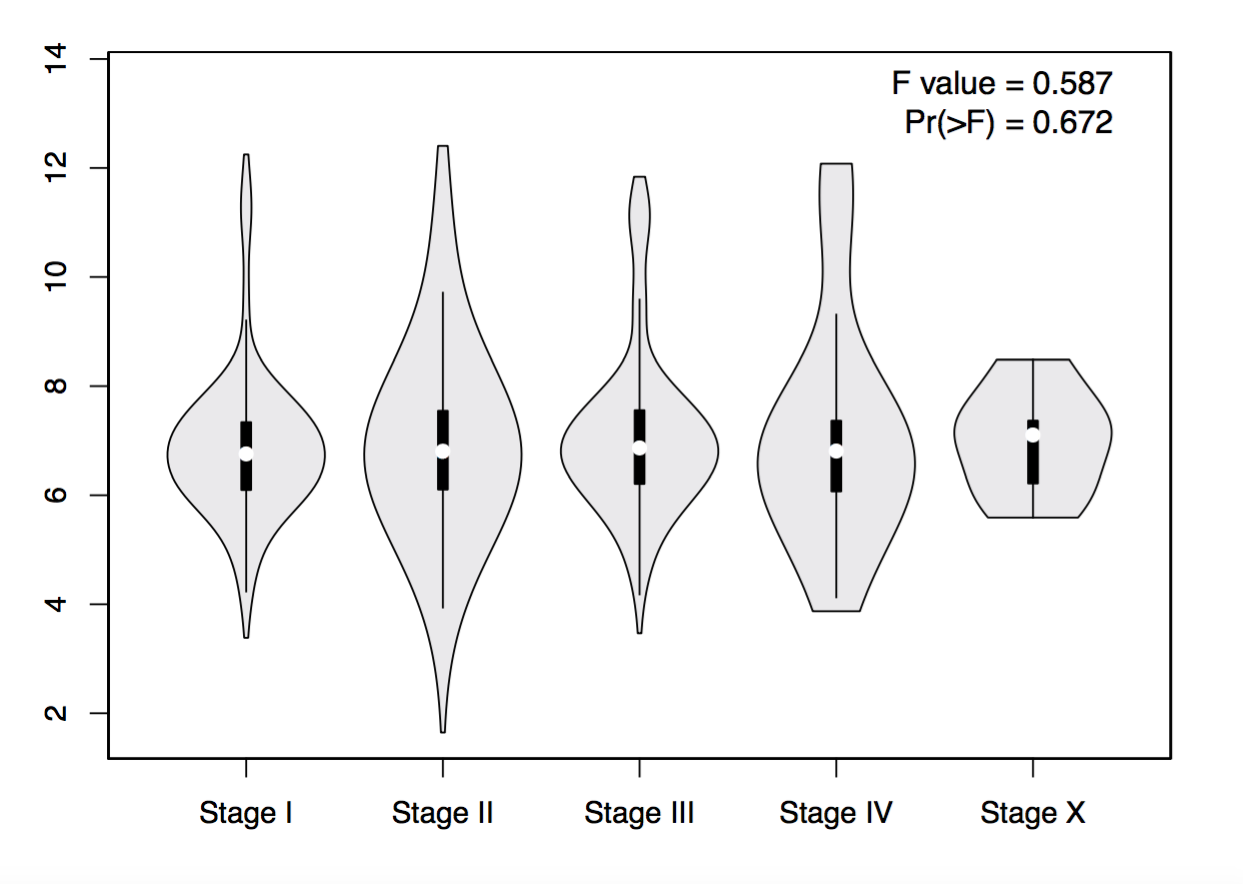
Profile based on pathological stage

This feature generates expression violin plots based on patient pathological stage.

Parameters

Gene: Input a gene of interest.
Datasets Selection/Dataset: Select one or multiple cancer types of interest in the “Dataset Selection” field and click “add” to build dataset list in the “Datasets” field. Manual input of cancer types split by comma (e.g. COAD,READ) is also acceptable.
Log Scale: Choose whether to use linear or log₂(TPM + 1) transformed expression data for plotting.
Use major stage: Choose pathological major stages or sub stages for plotting.
Plot Color: Set the violin color in the plot.

The method for differential gene expression analysis is one-way ANOVA, using pathological stage as variable for calculating differential expression:

Gene expression ~ pathological stage

The expression data are first log₂(TPM+1) transformed for differential analysis.

Notice: If only one sample exists in a certain stage, this sample will be filtered out by GEPIA to enhance the visual quality of the plot.

Results

Click the “Plot” button: GEPIA will generate a gene expression stage plot based on user custom inputs.

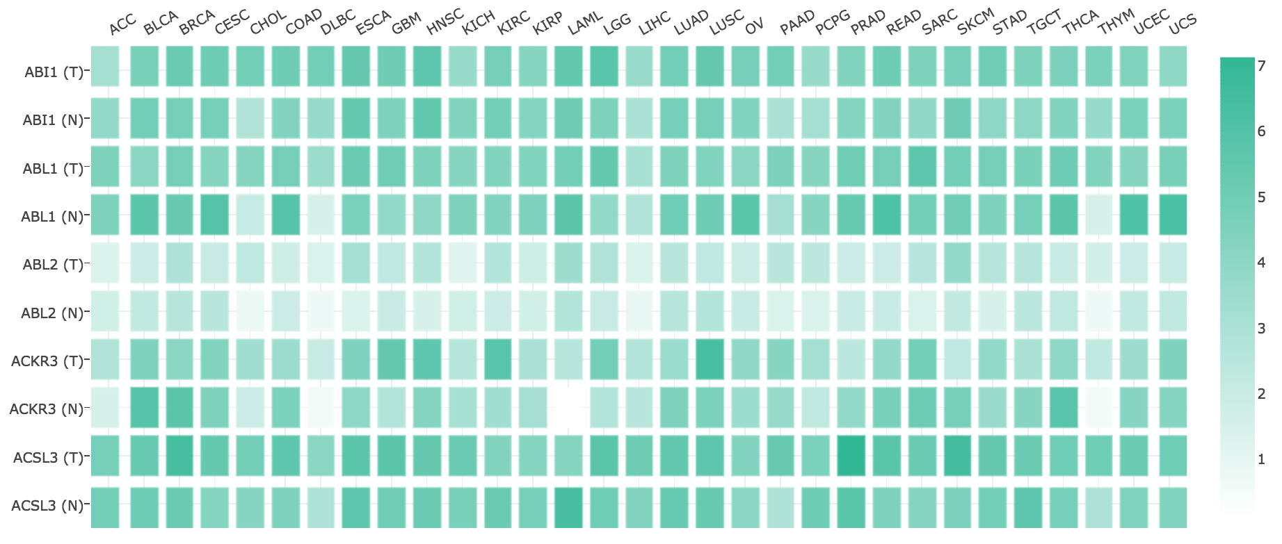
Multiple gene expression comparison

This feature provides expression matrix plots based on a given gene list. The density of color in each block represents the median expression value of a gene in a given tissue, normalized by the maximum median expression value across all blocks. Different genes in same tumors or normal tissues can be compared in one plot.

Parameters

Gene List: Input a gene list of interest. Manual input of genes split by comma (e.g. ERBB2,EGFR) is also acceptable.
Dataset/Tissue Order: Select cancer types of interest in the “Dataset” field and click “add” or “all” to build a dataset list in the “Tissue Order” field. Also, manual input of cancer types split by comma (e.g. ACC,BRCA,BLCA) is also acceptable.
Log Scale: Choose whether to use linear or log₂(TPM + 1) transformed expression data for plotting.
Matched Normal data: Select “Only TCGA tumor”, “TCGA tumor + TCGA normal + GTEx normal” or “TCGA tumor + TCGA normal” for plotting.

Results

Click the “Plot” button: GEPIA will generate an expression matrix plot based on user custom input parameters.

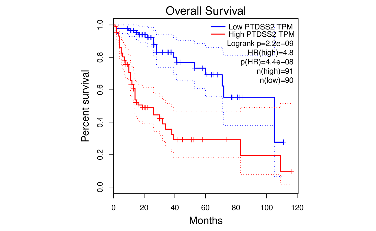
Survival Analysis

GEPIA performs overall survival (OS) or disease free survival (DFS, also called relapse-free survival and RFS) analysis based on gene expression. GEPIA uses Log-rank test, a.k.a the Mantel–Cox test, for hypothesis test. Cohorts thresholds can be adjusted, and gene-pairs can be used. The cox proportional hazard ratio and the 95% confidence interval information can also be included in the survival plot. Genes most associated with patient survival can be searched.

Parameters

Survival Plots

Gene: Input a gene of interest.
Normalized by gene: Set the gene used for normalizing in “Gene” field.
Methods: Select the OS or DFS survival method.
Axis Units: Select Month or Day unit for plotting.
Datasets Selection/Datasets: Select one or multiple cancer types of interest in the “Dataset Selection” field and click “add” to build dataset list in the “Datasets” field. Also, manual input of cancer types split by comma (e.g. COAD,READ) is also acceptable.
Color Reverse: Choose whether to reverse the default color.
Group Cutoff: Select a suitable expression threshold for splitting the high-expression and low-expression cohorts.
Cutoff-High(%): Samples with expression level higher than this threshold are considered as the high-expression cohort.
Cutoff-Low(%): Samples with expression level lower than this threshold are considered the low-expression cohort.

Most Significant Survival Genes

Datasets Selection: Select a cancer type of interest.
Methods: Select the OS or DFS survival method.
Group Cutoff: Select a suitable expression threshold for splitting high-expression and low-expression cohorts.

Results

Survival Plots

Click the “Plot” button: GEPIA will generate a survival plot based on user custom input parameters.

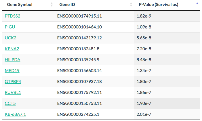
Most Significant Survival Genes

Click the “List” button: GEPIA will generate a list of top 100 most significant survival genes given a cancer type.

Similar genes detection

This function identifies a list of genes with similar expression pattern with an input gene and selected datasets.

Parameters

Gene: Input a gene of interest.
Top # similar Genes: List top # most similar genes. (Maximum: 200)
TCGA Tumor/TCGA Normal/GTEx/Used Expression Datasets: Select cancer types of interest in the “TCGA Tumor”, “TCGA Normal” or “GTEx" field and click “add” to build dataset list in the “Used Expression Datasets” field. Also, manual input of cancer types split by comma (e.g. COAD Tumor,READ Tumor) is also acceptable. The similar genes are detected based on the datasets list.

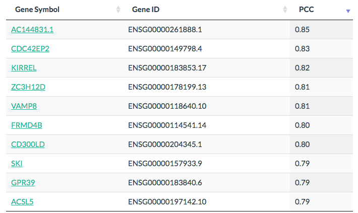
Results

Click the “List” button: GEPIA will generate a list of genes that have similar expression pattern ranked by Pearson correlation coefficient (PCC).

Correlation

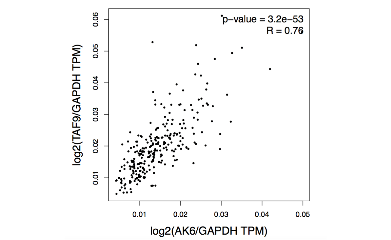
This function performs pair-wise gene expression correlation analysis for given sets of TCGA and/or GTEx expression data, using methods including Pearson, Spearman and Kendall. One gene can be normalized by other gene.

GEPIA uses the non-log scale for calculation and use the log-scale axis for visualization.

Parameters

Gene A: Input a gene A of interest. [For x-axis]
Gene B: Input a gene B of interest. [For y-axis]
Normalized by gene: Set the gene used for normalizing Gene A and Gene B.
Correlation Coefficient: The method for calculating the correlation coefficient.
TCGA Tumor/TCGA Normal/GTEx/Used Expression Datasets: Select cancer types of interest in the “TCGA Tumor”, “TCGA Normal” or “GTEx" field and click “add” to build dataset list in the “Used Expression Datasets” field. Also, manual input of cancer types split by comma (e.g. COAD Tumor,READ Tumor) is also acceptable. The correlation analysis is based on the datasets list.

Results

Click the “Plot” button: GEPIA will generate a scatter plot of correlation analysis result.

Dimensionality Reduction

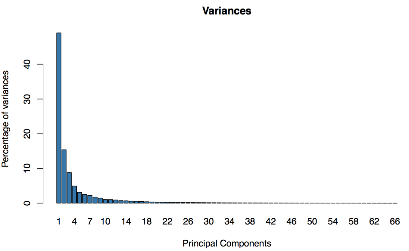
GEPIA performs Principal Component Analysis (PCA) for a given gene list using custom TCGA and/or GTEx expression data. First, GEPIA presents a 3D plot of top three principal components (PC) and generates a bar plot for variances interpreted by each PC. Second, GEPIA presents 2D plot or 3D plot based on user-specified PCs.

Parameters

First Step

Gene List: Input a gene list of interest. Manual input of genes split by comma (e.g. ERBB2,EGFR) is also acceptable.
Log Scale: Choose whether to use linear or log₂(TPM + 1) transformed expression data for plotting.
Scale: Choose whether to use Z-scores instead of the expression levels as input for PCA analysis.
TCGA Tumor/TCGA Normal/GTEx/Used Expression Datasets: Select cancer types of interest in the “TCGA Tumor”, “TCGA Normal” or “GTEx" field and click “add” to build dataset list in the “Used Expression Datasets” field. Also, manual input of cancer types split by comma (e.g. COAD Tumor,READ Tumor) is also acceptable. Principal components analysis is based on the datasets list.

Second Step

PC Selection: Select the PCs for 2D (set x and y values) or 3D scatter (set x, y and z values) plots.

Results

First Step

Click the “List” button: GEPIA will generate a 3D scatter plot and variance distribution based on the correlation analysis result.
The 3D plot can be saved as .png file by clicking the camera icon on the top-right.

Second Step

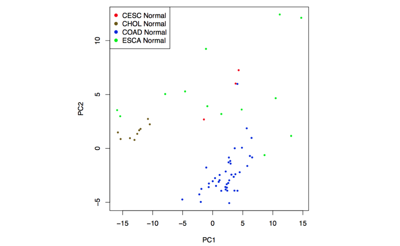
Click the “Plot 2D” button: GEPIA will generate a 2D scatter plot of the correlation analysis result.
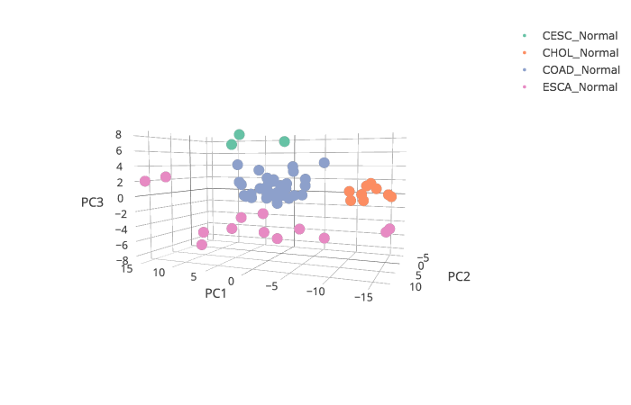
Click the “Plot 3D” button: GEPIA will generate a 3D scatter plot of the correlation analysis result.

Differential analysis

We use three methods for differential expression analysis using TCGA tumor samples with paired adjacent TCGA normal samples and GTEx normal samples.

Why do we use both TCGA normal and GTEx normal samples for differential analysis?

TCGA produced 9,736 tumor samples across 33 cancer types, while this project only provides 726 normal samples. The imbalance between the tumor and normal data can cause inefficiency in various differential analyses. Fortunately, GTEx project produced RNA sequencing data for ~8,000 normal samples. Meanwhile, UCSC Xena project recomputed the TCGA and GTEx raw RNA-Seq data using a standard pipeline, which makes two datasets compatible. As a result, the TCGA and GTEx data could be integrated for very comprehensive expression analysis.

we consulted with multiple medical experts to determine the most appropriate tumor-normal comparisons. The comparisons and data we used are presented below:

Differential methods

ANOVA

Considering the different stratifications of sex, age, ethnicity in tumor and normal samples, we applied four-way analysis of variance (ANOVA), using sex, age, ethnicity and disease state (Tumor or Normal) as variables for calculating differential expression:

Gene expression ~ sex + age + ethnicity + disease state

The expression data are first log₂(TPM+1) transformed and the log₂FC is defined as median(Tumor) - median(Normal).

The Benjamini and Hochberg false discovery rate (FDR) method was used to adjust the p-value in each factor to obtain the multiple testing adjusted q-value.

LIMMA

For an alternative method, we use the linear model and the empirical Bayes method implemented by the R package limma, with adjusted p-value (Benjamini and Hochberg FDR). The limma method leverages the highly parallel nature of genomic data, borrowing information between the gene-wise models.

Similarly, the expression data are first log₂(TPM+1) transformed and the log₂FC is defined as median(Tumor) - median(Normal).

Top 10

Cancer drug targets such as ERBB2, VEGF, are over-expressed in a subset (10-20%) of tumors and lowly expressed in all normal tissues. When discovering cancer drug targets, genes like ERBB2 and VEGF are ideal candidates as therapeutic targets. For this purpose, we implemented a method for detecting the genes that are over-expressed in only a subset of tumors for a given cancer type.

For each cancer type, we choose tumor samples that have the top 10% expression level for a given gene. For comparison, we choose the same number of normal samples that have the highest expression level for the same gene. We rank the tumor and normal samples by expression level and calculate the percentage of tumor samples in top 50% ranked list as the percentage value. The expression data are first log₂(TPM+1) scaled and the log₂FC is defined as median(Tumor) - median(Normal).

By default, we report the over-expressed genes as those passing following thresholds:

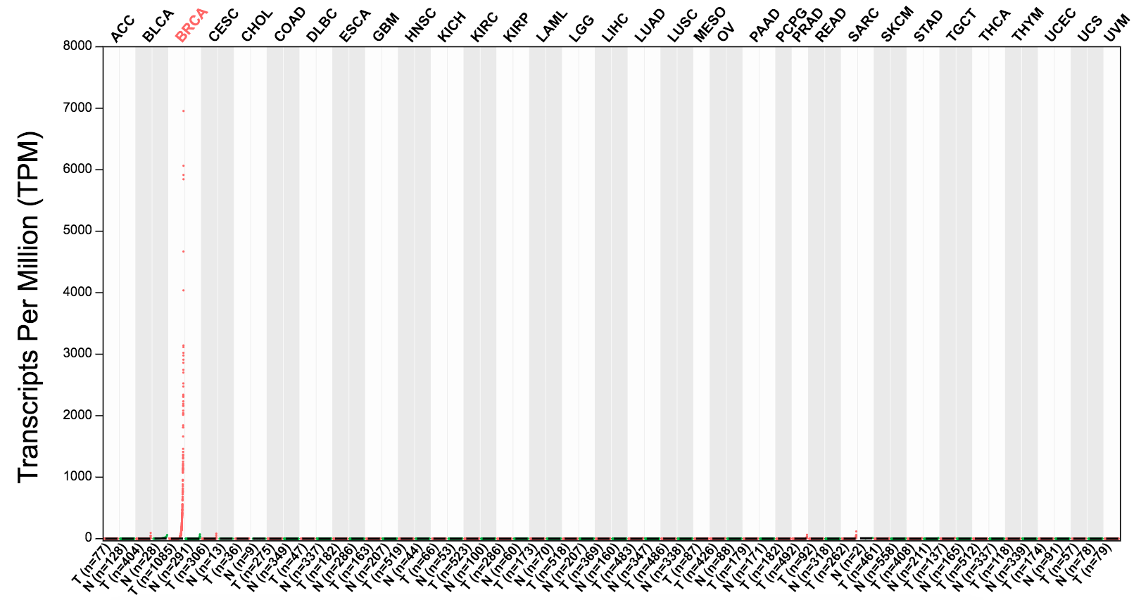
log₂FC > 1, percentage > 0.9.

For example, CLEC3A is over expressed in breast cancer and lowly expressed in all normal tissues as the profile below:

Definition of differentially expressed genes

For the ANOVA and LIMMA methods, genes with higher |log₂FC| values and lower q values than pre-set thresholds are considered differentially expressed genes.

For the Top 10 option, genes with higher log₂FC values and higher percentage value than the thresholds are considered over-expressed genes.

Results Download

The PDF and the SVG download is available by clicking the button nearby the results.

Edit Results

The downloaded PDF and the SVG plots can be edited by Adobe Illustrator. Here is a tutorial video:

Youtube (for global users)

Tencent (for Chinese users)